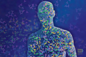
Go with your guts, and the billions of bacteria that are in them!
Test your own personal microbiome (or your pet’s) –
In this class you will be able to investigate your own gut microbiome, or the microbes of your pets, roommates, or family members. Our microbiome (the microbes living in and on our bodies) are believed to have profound effects on our immune systems, health, and susceptibility to disease. Find out what you can learn about your own health and wellness. In this class you’ll perform lab work to isolate the microbes present, sequence and identify those microbes, and then learn what the results mean for YOU personally.
In this 3 Saturday class you’ll be able to design your own experiment to compare any two samples! What samples do you want to compare? How many gut microbes you share with your dog? What about with another human? Does your gut microbiome change with your diet? What if you ate pizza for two weeks straight? (We do not endorse pizza as a sole source of nutrition!)
Isolate and process DNA from your samples. Use the polymerase chain reaction (PCR) to amplify the DNA of the microbes. Determine the different species of in your two samples. For those interested in programming and computational biology, the entire class will learn how to analyze the sequencing data and perform comparative analysis to uncover further information (don’t worry, this class is appropriate for beginners!).
Everyone gets two biological samples to test, here are some experimental suggestions. If none of these interest you, just ask us if you have another idea.
Some experimental suggestions:
1) Test your microbiome vs. your roommate (or friend, or family member)’s microbiome *
2) Test your microbiome vs. your pet **
3) Test your microbiome before and after a lifestyle change such as a change in diet, exercise or sleep habits
4) Test your pet microbiome before and after a change in your pet’s lifestyle
In the pursuit of knowledge in any field, a well-crafted introduction is a key element for eventual mastery of the subject matter. Unfortunately, when it comes to learning a new computer language, this element is missing from all too many first encounters. A failed initial coding experience, bedeviled by cryptic error messages for which no help is at hand, and perhaps accompanied by doubts that any useful application can be mastered in the near term, may be all that it takes to dash a beginner’s hopes and engender resistance to ever trying again. Happily for all concerned, BUGSS’s recent three-day course “Computational Modeling in Biology” followed a trajectory designed to ensure a successful learning experience.
Led by Johns Hopkins Ph.D.
candidate Wangui Mbuguiro and offered on three consecutive Saturdays, the
course was structured as an introduction to building mathematical models in the
R programming language for the analysis of biological data. In keeping with
this design, the focus was not on an exhaustive study of R and all of its
resources, but rather on how to employ some of the most powerful features of
this versatile language to accomplish common tasks in biological research.
Week 1: Deterministic Modeling
In the opening session March 2,
after guiding class members through the installation of R and the RStudio
integrated development environment on their laptops, Ms. Mbuguiro presented an
introduction to deterministic modeling. Each model considered was a mathematical
explanation of a biological process of interest. “Deterministic” means that the
output of the model depends solely on the precise values and conditions used as
input for the model, and not on any variables that may have a random or other
probabilistic distribution. The class
recreated deterministic models – expressed in R – for drug delivery via nanoparticles
and for bacteria grown in culture. We also explored fitting functions to our
data – that is, optimizing a model to best account for our data – using the
least squares method.
Rather than writing code from
scratch, we began by modifying short segments of existing code provided in the
development environment. This enabled us to avoid trivial mistakes and permitted
the focus to remain on gaining experience using mathematical concepts expressed
in R to study a biological system.
Week 2: Modeling growth rates
On the second Saturday, March 9, we
explored using R for a common laboratory task: calculating the varying rate of
change over time for a biological process involving a material of interest, and
using the results to obtain a close estimate of the quantity of that material which
is present at various time intervals. The
varying rates of change are values of an ordinary differential equation. Using these values to obtain numerical
approximations of the concentration of the material of interest at
different points in time can be
especially useful when direct analytic evaluation is difficult. In particular,
the class focused on modeling the growth rate of bacterial colonies. We started with the essential relationship
between the concentration of bacterial cells present and the growth rate of
that cell concentration when there are no external constraints, such as limits
on food supply.
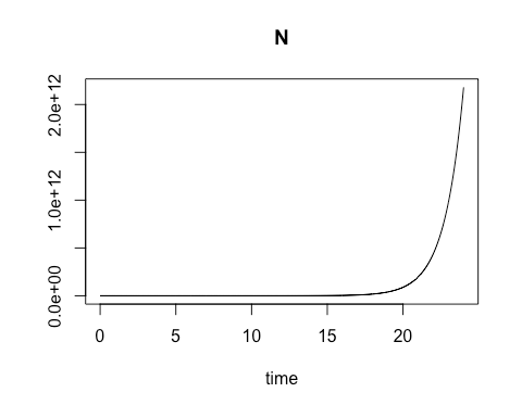
By calculating the rate of change
in cell growth over very small changes in time using a species-specific growth
rate constant and the concentration at the start of the time period, we were
able to estimate the cell concentration at each incremental time point. When
plotted, these cell concentration calculations formed a smooth curve that
revealed exponential growth over the time sequence.
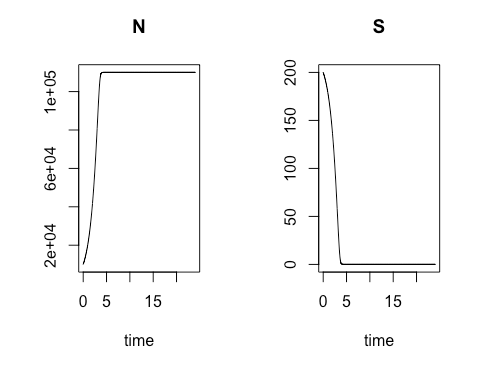
Next we altered the model to be
more reflective of real-world conditions. Relying on an equation developed by
Nobel-Prize-winning French biochemist Jacques Monod, we created in R the code
to calculate and chart both bacterial colony growth and the depletion of
nutritive media over time. As in the previous model, the colony growth rate is
dependent on the concentration of cells present at a given moment in time, but
in this model the natural increase in cell concentration is tempered by the
gradual depletion of the cells’ nutritional medium, or substrate, at a variable
rate which also depends on the concentration of cells present. We again used
R’s plotting package to graphically display the cell concentration N and for
the substrate concentration S over time.
Week 3: Sensitivity Analysis
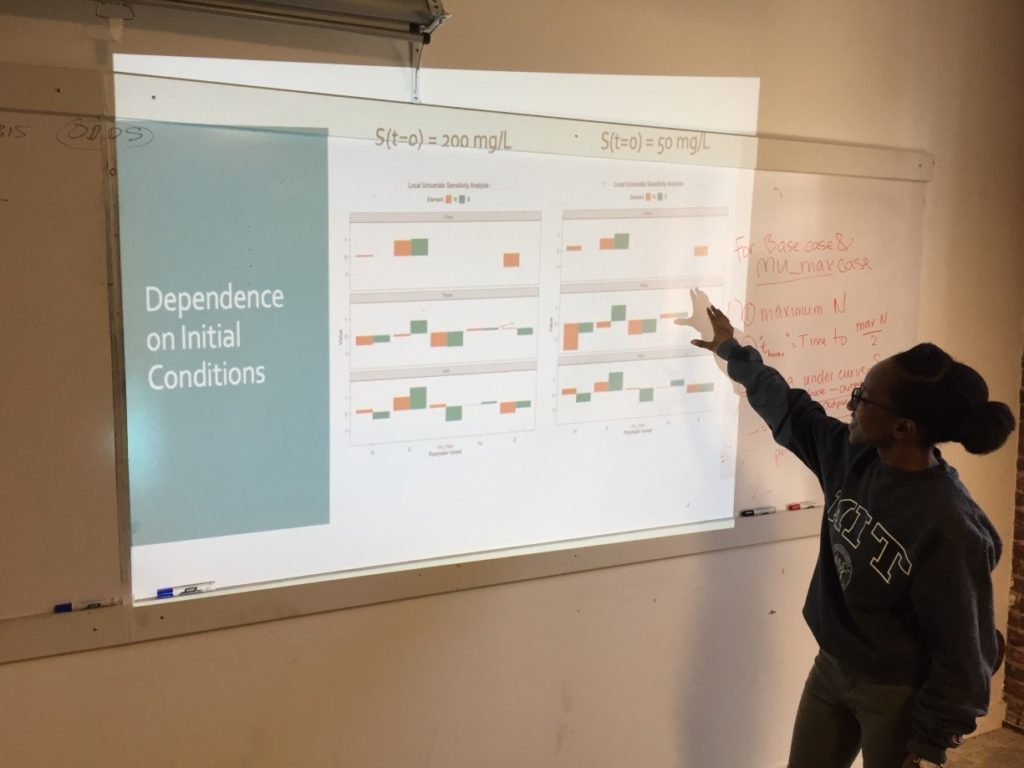
On the third Saturday, March 16, we
conducted a sensitivity analysis on the Monod model of cell concentration
increase and substrate depletion. Creating code in R for changing – one at a
time –each relevant initial condition of the system and each rate-governing
parameter, we explored the effect on the final outputs – cell concentration and
substrate concentration – of a 10% change in each of the initial conditions and
parameters.
Looking at the effect of a 10%
increase in the growth constant, we learned how to get a close estimate of the
time required to reach half of the maximum cell concentration. As an
illustration of how easily R can accommodate new functions to meet special
needs, Ms. Mbuguiro wrote a “helper function” to find the position number
within a sequence of time values of the particular value associated with a cell
concentration that had reached 50% of the maximum.
The calculation of all output
changes driven by an incremental change of one input parameter is called a
univariate sensitivity analysis. Extending
our exploration of R for standard statistical manipulations, we normalized the
outputs of the entire sensitivity analysis – that is, we converted the change
in each output from an absolute measure into a measure that is relative to the
10% change of the growth constant.
As a last step, the class wrote the R code to create a graphical representation of the normalized output for multiple univariate sensitivity analyses, showing the effect of 10% changes in various parameters, considered one at a time, upon properties associated with cell concentration (N) and with substrate concentration (S). These properties include: Cmax, the maximum cell or substrate concentration; Thmax, the time required to arrive at one half of Cmax; and the Area under Curve (AUC), a measure of concentration over time that can be used to calculate average concentration during the time period. The area under the curve for the substrate concentration is often used in drug development research as a measure of “exposure” to the substrate. As an aid to visualization, the class made use of another R “helper function” contributed by Ms. Mbuguiro called output_calculator2, which works in concert with other R functions to produce the final output.
Although each Saturday session was
four hours long, the time passed quickly as we alternated between discussion of
applications and the production of error-free code. The classes were further
enriched by discussion of work by Birgit Schoeberl[1]
and Iraj Hosseini[2]
demonstrating how synthetic biology techniques such as model optimization and
sensitivity analysis can be used to design and implement drug therapies to
treat cancer and HIV, respectively. We
also benefited from review of a textbook chapter by Raina Maier[3]
that explains the utility of the Monod model and the mathematical tools of
synthetic biology for the large-scale production of microbial products including
antibiotics, yeast, and alcohol.
By the end of the last day, we
realized that we had been equipped with a powerful tool for setting up and
running our own models. Yet we also knew that we had barely scratched the
surface of the potential for using R to gain insight into biological data. We
departed with gratitude for the collective learning experience, and eager to
learn more.
– Mark V.
About the Instructor
Wangui Mbuguiro is a Ph.D. candidate in the Biomedical
Engineering Program at Johns Hopkins. Her research and passions center on
engineering tools to better understand and treat menstrual disorders as part of
the Computational Design of Therapeutics Lab. Outside of
lab, Wangui enjoys encouraging scientific inquisition as an instructor and
mentor at the Baltimore Underground Science Space, as well as building
opportunities and community for underrepresented students in STEM at Johns
Hopkins. Lastly, Wangui is a MIT alumna (B.S., Bioengineering, 2017), National
Science Foundation Fellow, and friendly neighborhood scientist. You can connect
with her on twitter (@WanguiMbuguiro)
or LinkedIn.[1]
Schoeberl, B. et al., Systems biology driving drug development: from design to
the clinical testing of the anti-ErbB3 antibody seribantumab (MM-121). npj Systems Biology and Applications
(2017) 3, 16034; doi:10.1038/npjsba.2016.34; published online 5 January 2017.
[2] Hosseini, I. and Mac Gabhann, F., Mechanistic Models Predict Efficacy of CCR5-Deficient Stem Cell Transplants in HIV Patient Populations. CPT Pharmacometrics Syst. Pharmacol. (2016) 5, 82–90; doi:10.1002/psp4.12059; published online 16 February 2016.
[3] Maier, R.M., Bacterial Growth. In Environmental Microbiology (Maier, R.M., Pepper, I.L., and Gerba, C.P., eds., 2nd ed., Academic Press, 2009), Ch. 3, p. 37-54. https://doi.org/10.1016/B978-0-12-370519-8.00003-1. (http://www.sciencedirect.com/science/article/pii/B9780123705198000031)
This class taught the fundamental techniques of molecular biology (PCR, restriction digest, ligation, and transformation) by cloning a regulated version of the holin gene which can then be activated to destroy bacteria.
Week 1
This week we performed PCR and gel electrophoresis and discussed what kill switches are.
Week 2
This week we performed Gibson Assembly and bacterial transformation and discussed bacterial toxin/antitoxin systems.
On the news, we often hear that certain genes have been linked to different traits, ranging from height, to body-mass-index, to heart disease risk. Curious about how these associations are discovered?
In this course, we learned all about the science behind the studies. We learned about basic genetics and genomics and even some statistics. Check out the recordings, and thanks so much to Stephanie Yang for a fantastic class!
Session 1
Session 2
Session 3
Want more info on how linear regression works and how changing the parameters affects the outcome? Check out Stephanie’s Linear Regression App!
Modern neuroscience, despite being about 110 years old, is quite young compared to other fields of science. In 1906, Spanish neuroscientist, histologist, and pathologist Simon Ramón y Cajal collaborated with Italian biologist Camillo Golgi (the namesake of the Golgi Apparatus) in an attempt to study the structure of “brain cells” while making use of a technique for creating a color contrast between cellular components called Golgi staining. This effort earned the pair the 1906 Nobel Prize in Medicine, and Ramon y Cajal the title of “The Father of Modern Neuroscience”.
One major finding from the two was that the brain and what we know today as the Central and Peripheral Nervous Systems (CNS, PNS) are made up of billions of individual cells called “neurons”. Each neuron has four major parts. The dendrites receive information from other neurons. However, the dendrites themselves don’t do the receiving – that’s done by little structures called dendritic spines, which are prone to frequent change. Next up is the soma or the cell body. The axon and axon terminal pass the impulse along through a mechanism called saltatory conduction. The axon terminal transmits the signal to the next neuron’s dendrites across a gap called the synaptic cleft, and the cycle continues until the impulse reaches the desired location or is inhibited (or canceled).
The synaptic cleft is quite interesting, as it is perhaps one of the most flexible areas of neuronal growth. As we learn more and commit lessons to memory, we use some neuronal pathways (and therefore those synaptic clefts) more than others. We call this concept “synaptic plasticity”, the modification of players in the synaptic cleft under increased or decreased usage. Synaptic plasticity is so important in building memory and for a properly maturing nervous system that deficits in synaptic plasticity have been linked to Alzheimer’s disease, intellectual disabilities, autism, and schizophrenia. With such an important biological tool at its disposal, the cell has put it to use with an equally skillful operator – the AMPA receptor, or AMPAR.
To learn what role AMPA (a compound with a very long name) and its receptor play in memory-making, learning, and synaptic plasticity, we hosted a seminar on 9/19/2020 featuring Dr. Elena Lopez-Ortega. She also discussed microscopes and how we can use different types of microscopes to study neuronal cells, synapses, and receptors as they change as a result of synaptic plasticity.
Check out the recording to learn more about the evolution of microscope design, optical microscopes, confocal microscopes, fluorophores, and ways to make a sample easier to investigate. She also introduces software that you can use to try your hand at analyzing some specimen data!